
Digital Nose - Phase IV: Building the Odour Dataset
Phase III of Digital Nose ended with a better way to preserve sensor data. The raw measurements had their own storage path, the database handled the application, and sensor health became part of the dataset. Two BME690s were still on the same heater setting. Their gas-resistance traces followed similar shapes at different absolute levels, which is useful for comparing the sensors, but it does not use the heater-temperature scan the BME690 can do. Before adding more hardware, I wanted to see what those sensors could capture when the frying smell from the nearby restaurant was noticeable.
For Phase IV I capture a smell on purpose: record the heater settings, write down what I smelled, and check the traces before using them for training. Doing that turned up two compensation bugs in the BME690 driver, and it changed how a capture is recorded.
Moving from continuous collection to deliberate captures
Phase III preserved the continuous raw stream so I could investigate the instrument without discarding potentially useful information. For Phase IV, the BME690s, SGP41 and SPS30 run only during confirmed manual captures. The original ENS160 still operates continuously. Its TVOC, eCO₂ and AQI readings remain on the main dashboard, alongside smell reports, window and occupancy context, weather and wind history.
When I notice a smell, I open the capture form, describe the observation and confirm the request. The microcontroller receives the command, prepares the sensors and starts a two-minute recording. Preparation takes about two minutes as well. Both periods are choices for this project. They are not Bosch requirements, and they are not a claim that this timing suits every smell. Between captures the array stays idle. Device health, command polling and pending uploads continue, but those sensors no longer produce a continuous environmental stream.
Each capture then has a start time, a heater configuration, and a written observation, whether that is restaurant frying or ordinary room air. Manual capture still introduces selection bias, because I choose when to record. The first dataset describes those selected observations. Testing a detector that runs all the time will need broader data. The first question is whether restaurant-like frying looks different from ordinary air when I record both the same way.
One reference sensor and one temperature scan
The two BME690s now have different roles. BME690 #1 keeps the fixed reference setting of 320°C with a 150 ms heater duration. BME690 #2 cycles through five configured heater temperatures:
| Step | Heater target | Heater duration |
|---|---|---|
| 0 | 200°C | 150 ms |
| 1 | 250°C | 150 ms |
| 2 | 300°C | 150 ms |
| 3 | 350°C | 150 ms |
| 4 | 400°C | 150 ms |
These temperatures refer to the internal gas-sensing hotplate, not the ambient temperature measured by the sensor. The software selects a heater step, requests a forced measurement, records the result and moves to the next step. A complete scan produces five gas-resistance measurements. Changing the hotplate temperature changes how the sensing surface responds to the surrounding gases.
It does not make the sensor a chemical analyser. This is an exploratory project configuration, not HP-354, a trained Bosch classifier or a profile already validated for frying fumes. I want to see whether the five-step pattern differs between ordinary air, restaurant-like frying, and other smells.
Different temperatures need separate charts
The first scan showed why the readings could not be combined into one resistance line. During an ordinary-air commissioning capture, BME690 #2 produced median resistance values ranging from approximately 1.22 MΩ at 200°C to 95 kΩ at 400°C. Joining those readings into one chart would create large jumps every time the heater setting changed, and those jumps would mostly describe the measurement sequence. The capture report therefore shows each heater step separately.
Every measurement retains its step index, cycle index, configured temperature, heater duration and validity information. Partial cycles are kept too. If recording starts halfway through a scan, the earlier steps are not invented or renumbered. The report stays compact, with small charts for each measurement. The complete JSON export contains the underlying data and settings for analysis.
Preparation does not guarantee a stable baseline
The first full tests used about two minutes of preparation followed by two minutes of recording. The hardware checks passed. The sensors reported fresh data, valid gas measurements and stable heater operation, but the gas-resistance traces were still rising. In one commissioning run, the reference BME690’s recording median increased by more than 50%. The scanning sensor also showed substantial changes within individual heater steps.
A stable heater means the hardware reached its operating condition for that measurement. It does not mean the gas response has stopped changing. This shows up when the sensors have been idle. Their recent heater history affects the reading, and the air in the room can change during the same two minutes. I kept all preparation and settling measurements. They are hidden in the default report, but an Include startup switch makes them visible. I also record the time since the previous capture, because a sensor restarted after a short pause may behave differently from one that has been idle for several hours.
Captures use the same bounded preparation procedure. I have not added a rule that waits indefinitely for a flat signal. A real odour changing in the room could prevent that condition from being reached, so I record the startup instead of waiting for a flat trace and then throwing those samples away.
A pressure difference exposed a driver fault
The ordinary-air test revealed a separate problem. Temperature and humidity agreed reasonably well. Pressure did not: the two sensors differed by about 9.09 hPa. The installed bme690 driver decoded one pressure calibration coefficient using the wrong byte from the sensor’s calibration data. Each sensor has its own factory calibration values, so reading the wrong byte affected the two sensors differently and looked like a physical offset.
Correcting the decoding and recalculating live readings reduced the pressure difference to approximately 0.18–0.21 hPa. No arbitrary offset was added to force agreement. The same audit found another compensation defect. The humidity calculation used par_h1 where Bosch’s implementation specifies par_h3. Its effect on the inspected readings was much smaller, around 0.17 percentage points of relative humidity, but it still needed correcting. This also affected the SGP41 indirectly, because its measurements use temperature and humidity from BME690 #1 for compensation after the initial conditioning period.
The gas-resistance calculation and heater-calibration paths did not use those faulty pressure and humidity calculations. The audit also found that the continuous ENS160 process needed to participate in the shared bus lock, so complete sensor operations could not interleave unexpectedly. The earlier captures remain intact, with quality flags describing the known issues. New captures use a versioned configuration identifying the corrected compensation code. The numbers looked plausible. The calibration decode did not. Checking the driver mattered as much as checking the sensors.
Making sure capture really stops
The 400°C heater target prompted another check: what happens when the capture ends? Both BME690s use bounded forced measurements. After each session, the worker places them into sleep mode, disables gas measurement and disables the heater, then reads the registers back to verify those states. Cleanup happens before pending uploads are drained, so a slow network cannot keep acquisition running past the local capture deadline.
SGP41 heater-off and SPS30 stop commands are also sent. Their installed interfaces do not provide the same independent state readback, so the records distinguish commands issued from shutdown states verified. Completion, early cancellation, worker termination and restart recovery were tested. Collected measurements remain in a durable local queue if they cannot be uploaded immediately. Two complete commissioning captures also verified that the sensors could finish a session, shut down and initialise successfully for the next one.
Labels need to describe what happened
A button press is not enough, because the smell can disappear during preparation, change during recording, or mix with another source. The capture form now separates the purpose of the session from the observed odour.
The observation choices are:
- Restaurant-like frying or oily odour
- Other odour
- No noticeable odour
- Unsure or mixed
Commissioning tests are recorded separately. Intensity is optional. A missing score remains unknown, rather than being treated as zero. Suspected source is stored separately, because recognising a smell does not establish where it came from.
During capture, I can timestamp when the smell changes or disappears. Afterwards, I can confirm whether it stayed the same throughout, changed or was uncertain. Several captures from one continuing nuisance can share an episode. Neighbouring measurements from the same episode should not be split between training and testing and presented as independent examples. The raw measurements and annotation history remain intact, so a later correction to a label does not erase what was originally recorded.
The first labelled captures
With the capture workflow deployed and the compensation faults corrected, I started collecting observations during noticeable cooking odour. On 1 October, I recorded four sessions labelled restaurant-like frying or oily odour. Each contained about two minutes of recording, with perceived intensity scores of four or five out of five. The capture history connects each timestamp and label to a specific set of sensor measurements.
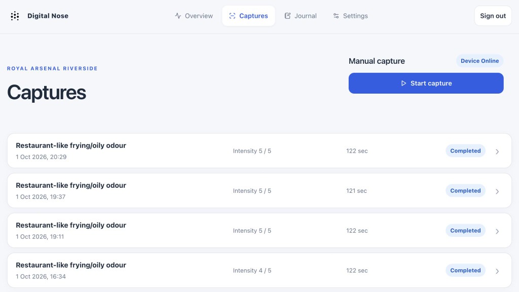
The first four completed odour captures, with observation times, perceived intensity and recording duration.
Opening a capture shows what I observed alongside what the sensors recorded. The evening session shown below contains 395 stored samples, of which 370 are marked valid. It is labelled as an observation, includes a suspected source and episode reference, and records my confirmation that the smell stayed the same throughout. The label describes the frying smell I noticed. The restaurant attribution remains my observation, not a conclusion produced by the sensors.
The report places the SGP41 gas responses, SPS30 particle readings and BME690 measurements together. In this session, the raw VOC response rises, the raw NOx response falls, and the particle traces show a brief excursion. Temperature changes very little. Those patterns are worth keeping, but one capture cannot establish which changes belong to the odour. They need comparison with ordinary air, other smells and repeated observations under different conditions.
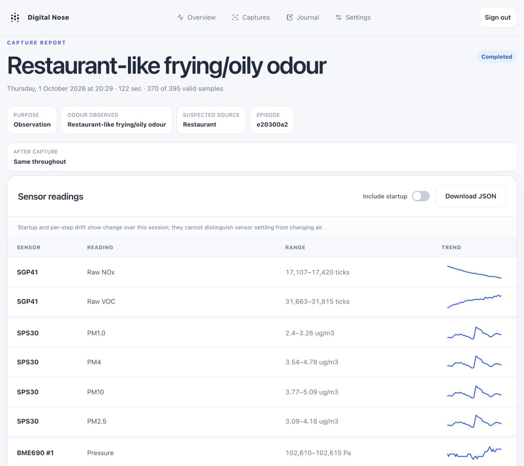
A completed capture connects the observation and persistence confirmation to the recorded sensor traces.
The second part of the report shows the fixed BME690 reference and the five separate heater-step responses. Keeping those readings separate lets me compare each temperature across captures. The traces also continue rising during recording, so startup behaviour remains part of the analysis. The charts are only a check. The JSON export has the samples, heater settings, and timestamps.
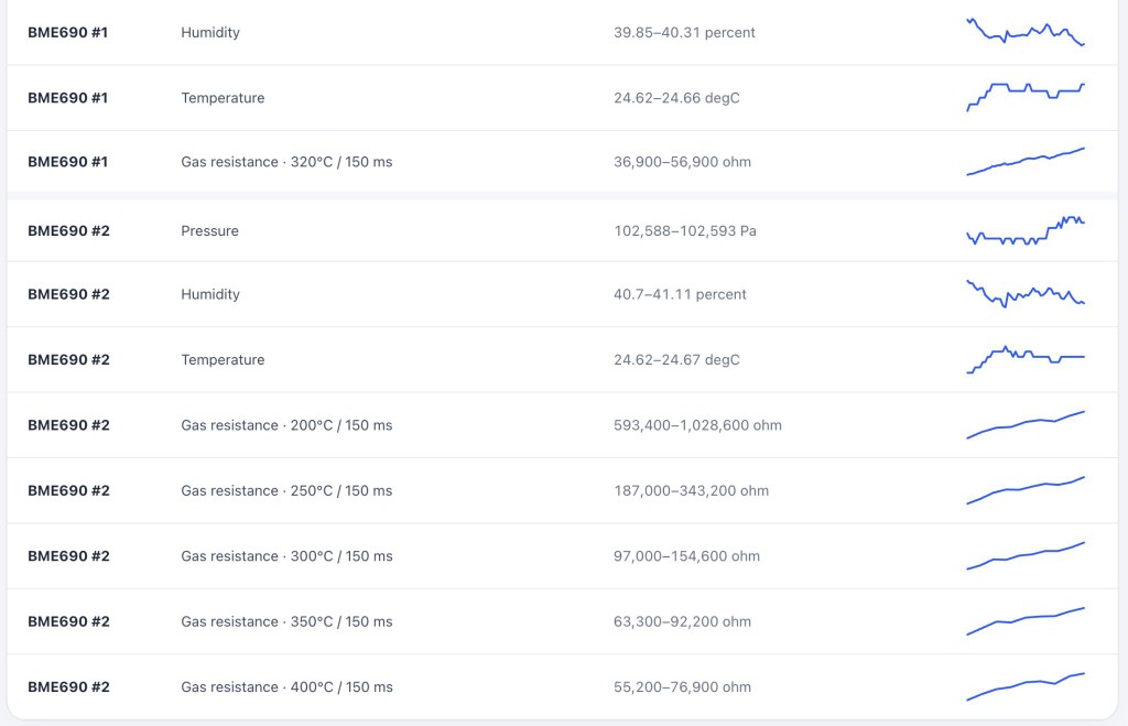
The 320°C reference and five experimental heater-step traces, preserved separately for comparison between captures.
Ordinary air is part of the experiment
I also need captures with no noticeable odour, and captures of other smells, including ordinary room air, indoor cooking and food. Otherwise, a model might learn to distinguish any gas response from quiet air rather than recognise the pattern I am interested in. The same applies to context. If every negative capture happens overnight and every positive capture happens during the afternoon, time, humidity or ventilation could become shortcuts. “No noticeable odour” is a useful human observation. It is not proof of chemically clean air.
The first comparison will use captures from the same sensor location and configuration, with startup history and environmental context retained. I need to see how much ordinary-air responses vary before deciding whether an odour response is different. The initial model target is limited to a response associated with the restaurant-like frying odour I observe at this location. Identifying the source independently, or measuring individual pollutants, would require additional evidence.
Where Phase IV leaves the project
Manual capture, the heater scan, labels, JSON export, and the shutdown check are running. The compensation bugs are fixed, and the older captures keep their quality flags. Training has not started. Next I need the same kind of capture on other days, including ordinary air, so a repeated frying session can be compared with something else. Phase V will add a separate physical array for simultaneous profile comparison. Repeated scans within one capture provide detail, but they do not replace independent observations.
Digital Nose is a Physical AI project: sense the real world first, then decide whether a model belongs in the loop. More on my profile.
Digital Nose · Open-source repository · Phase I · Phase II · Phase III