
Digital Nose - Phase III: Building the Dataset Before the Model
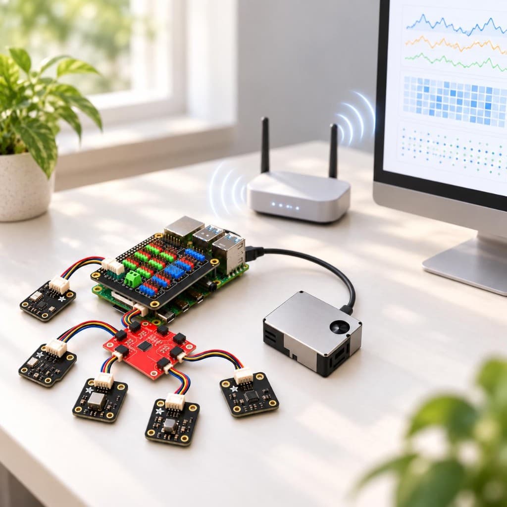
Digital Nose is an electronic nose: a gas sensor array for machine olfaction, not a single air-quality number.
Phase II of Digital Nose ended with a simple plan: leave the full sensor array running, collect calibration data and resist the temptation to train a model until I understood the instrument. Two BME690s were producing gas-resistance and environmental measurements at roughly one-second intervals, the SGP41 was producing raw VOC and NOx responses at about the same rate, the SPS30 was measuring particulate matter every few seconds, and the original ENS160 pipeline from Phase I was still running alongside them.
So I did. Within days, that exposed the next problem. The sensors were producing useful data, but I was storing it in the wrong place.
Phase I established that the phenomenon could be measured. Phase II built a more trustworthy multi-sensor instrument. Phase III is about making sure the resulting data is trustworthy enough to train on.
The first issue appeared almost immediately: the database was growing much faster than expected.
So the first Phase III problem was not model training at all. It was the data pipeline: how to keep high-frequency sensor data without turning the database into a permanent raw telemetry archive.
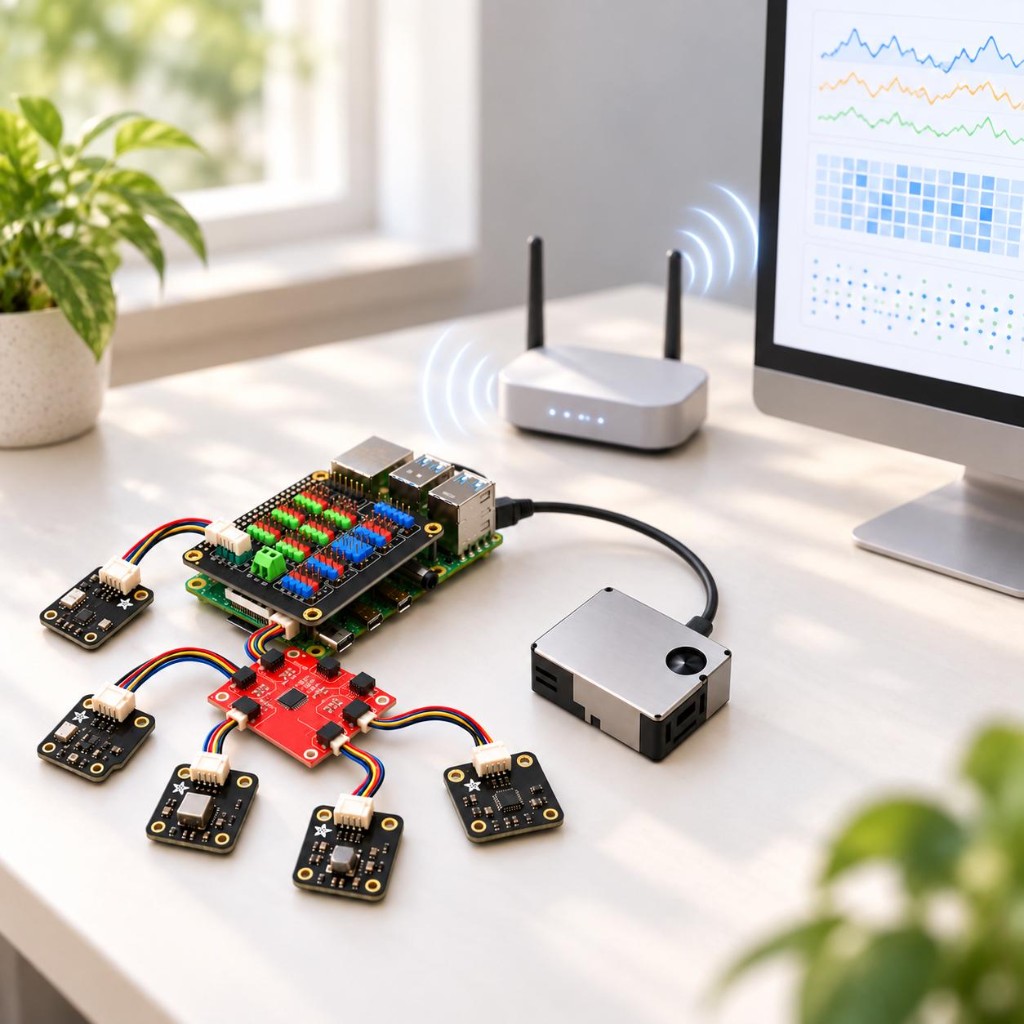
The array on the desk, a path onto the network, and a dashboard at the other end. Phase III leaves the sampling rate alone and changes what happens after each measurement.
The sensors were producing a lot of data
A 1 Hz sampling rate does not sound excessive until several sensors run at that rate continuously for days.
The two BME690s and the SGP41 were each generating about one observation every second. The SPS30 added another observation roughly every three seconds. Each measurement eventually became its own database row.
During the Phase III audit, the raw observation table had already passed 880,000 rows. It later exceeded 1.3 million rows and occupied more than 1 GB once indexes were included.
Three sensors at one sample per second is 3 × 86,400 = 259,200 observations/day. The SPS30, at about one sample every 3 seconds, adds 28,800 observations/day. Together that is about 288,000 raw observations/day, roughly 8.6 million a month and 105 million a year.
The exact rate varies, but the direction was clear: this was not a temporary quota problem. At the existing sampling rates, the architecture itself had to change.
Nothing was broken; the system was behaving as designed. The design simply did not scale well for continuous acquisition.
In Phase II, the database was doing two jobs: serving the application and storing every raw sensor observation. That worked well for the prototype, but it was not a sensible long-term storage model for a continuously running sensor system.
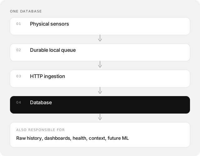
All data paths ended in the same database. It was handling both live application queries and millions of raw measurements that were rarely updated once written. Those two workloads needed to be separated.
More data is useful only if it has the right context
For physical sensing, I still want to preserve the raw signal whenever possible. High-frequency data contains timing information that can disappear if it is aggregated too early. The question is where to keep it.
The database is useful for things I query constantly: recent summaries, sensor health, smell reports, weather context, labels, experiment state, and eventually model outputs. Millions of one-second raw observations are a different workload. They are raw sensor telemetry rather than normal application data.
That distinction also matters for the future ML pipeline. Storage size was only part of the problem. The dataset also needed enough context to show whether each period of data was trustworthy.
Missing data is ambiguous. A gap can mean normal air, a sensor failure, a restarting worker, network loss, publishing delay or an intentional pause. If those states are not recorded explicitly, they can easily be misinterpreted during training.
Phase III therefore had two goals: preserve the raw signal efficiently and record enough sensor health to know whether the data is valid.
Why I did not reduce the sampling rate
The simplest fix would have been to lower the sampling rate. For example, the 1 Hz sensors could have been reduced to one sample every 10 or 60 seconds, or replaced with rolling averages. I chose not to do that.
For odour detection, the useful signal may be temporal rather than absolute: which sensor responds first, how quickly it rises, how long the response lasts and how different sensors move relative to each other. Reducing the sampling rate too early could remove the timing information that SSM may later need. A one-minute average alone is also insufficient. A short 10-second spike can be heavily diluted by the remaining 50 seconds of normal readings.
The resulting design principle was simple:
Acquisition cadence and storage cadence do not have to be the same thing.
The sensors can keep their native sampling rates while the database receives only the summaries needed by the live system. The raw stream can be archived separately.
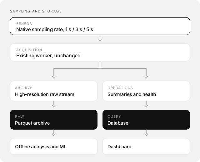
That separation became the basis of Phase III.
Separating raw storage from the live database
The existing acquisition workers could stay unchanged. Phase II already had independent workers, durable queues and retry logic, so there was little reason to disturb that part of the system. The problem was storage, not acquisition.
Phase III therefore added a preservation layer after acquisition. For the migrated sensors, raw full-resolution data is now stored outside the database. The database receives one-minute summaries containing the minimum, maximum, mean, sample counts and coverage information.
A simplified summary might look like this:
{
  "sensor_key": "bme690_1",
  "minute": "2026-09-26T18:42:00Z",
  "sample_count": 60,
  "valid_count": 60,
  "missing_count": 0,
  "temperature": {
    "min": 22.81,
    "mean": 22.93,
    "max": 23.04
  },
  "gas_resistance": {
    "min": 84210,
    "mean": 86144,
    "max": 88930
  }
}
This is simplified, but it shows the structure. The application can now represent that minute with one summary row instead of roughly sixty raw rows. The underlying raw measurements are still available in the archive. Keeping the minimum and maximum also preserves short excursions that an average alone could hide.
Moving raw telemetry to Parquet
Parquet is a better fit for this type of append-only telemetry. The access pattern is almost the opposite of an application database. Raw observations are append-only, rarely updated individually, and later read in large time ranges for analysis or training. Typed, compressed, columnar Parquet partitions fit that workload much better than millions of individually indexed database rows.
Once a measurement has been captured, it rarely needs to change. It mainly needs to be stored reliably and read back efficiently for analysis or training.
Phase III now stores the full-resolution stream as typed Parquet files. The archive retains original timestamps, sequence information, readings, sensor state and provenance, meaning the software, configuration and session that produced the measurement. Each archive part also has manifest metadata and SHA-256 integrity checks.
The database handles live queries and summaries. Parquet stores the raw history.
Why adaptive capture has to wait
The original Phase III design used adaptive capture. The idea was to keep a lower-volume baseline and switch to full-resolution capture when an event was detected, followed by a recovery window: baseline, then triggered, then recovery.
I still expect to use that model later. I decided not to implement it yet because it could bias the training dataset. If the anomaly trigger is designed before the sensor distribution is understood, it starts deciding which samples are retained. That would bake my assumptions about interesting events into the dataset before the model has had a chance to learn the real patterns. In ML terms, this introduces selection bias: an unvalidated detector would decide which parts of the underlying data distribution the future model is allowed to see. Effectively, the trigger would censor the training distribution using a rule that has not itself been validated.
A weak plume might never cross the trigger, slow changes could be lost, and quiet periods could become underrepresented. The model could then appear accurate on a dataset that had already been filtered by the same assumptions.
So I changed the order of work. For now, the system keeps the full-resolution stream during the restaurant-relevant window, currently 10am to 11pm. Adaptive capture will come later, once I have enough real data to define and test the trigger properly. For the first training dataset, I would rather over-collect into cheap storage than discard useful examples too early.
Health became part of the dataset
Phase II also showed that sensor health has to be stored alongside the measurements. It affects how the data should be interpreted.
For example, a training window may contain a stale SGP41, a recovering BME690 and missing SPS30 data. Without health metadata, that window could be mistaken for an unusual environmental event. In reality, the sensor system was unhealthy.
Phase III now records expected and observed samples, invalid or missing readings, worker freshness, queue state, disk capacity, archive state and clock synchronisation.
A future training pipeline can therefore reject or flag unhealthy windows:
if window.device_health != "healthy":
    exclude_from_training(window)
The real rule will be more nuanced, but the basic idea is simple. Both can look like nothing happened, but only one represents valid baseline data.
Archive-only mode
After the archive path was verified sensor by sensor, the high-frequency publishers were switched to archive_only mode. Conceptually, the flow is:
observation = queue.next()

preserve_raw(observation)

if preservation_succeeded:
    acknowledge_local_queue(observation)

    if publish_mode == "normal":
        send_to_database(observation)
    elif publish_mode == "archive_only":
        pass
The ordering matters: raw preservation happens before the original queue item is acknowledged. If preservation fails, the queue entry remains and can be retried. This reduces database writes without weakening delivery guarantees.
SGP41 was commissioned first, followed by BME690 #1, BME690 #2, and finally the SPS30. The ENS160 stayed on its existing minute-aggregation path, which was already efficient.
Database growth dropped immediately
The three ~1 Hz streams alone produced ~260k database rows per day. Switching them to archive_only stopped those raw writes without changing the sampling rate. The SPS30 then moved to the same setup.
I also removed older Phase II raw rows that were no longer needed in the database. Once archive coverage had been verified, ~1 million older raw observations from the two BME690s, the SGP41 and the SPS30 were removed. Newer observations and the context tables stayed.
One PostgreSQL detail was worth noting: deleting almost one million rows did not reduce the physical file immediately. Normal VACUUM lets the database reuse that space, but it does not necessarily return the allocated pages to the filesystem. The raw table still occupied roughly 1.18 GB after the logical cleanup. A later physical rewrite, such as pg_repack, can reclaim that space properly. The key result is that the table can reuse freed space and the high-frequency raw writes have stopped.
Phase II vs Phase III
Phase II treated the system roughly as sense, upload, store a row, and repeat. Phase III treats the same measurement as something that has to be preserved, then split into a raw archive, an operational summary, and a health record.
The change is architectural, not just a storage cleanup. Raw measurements are now treated as training and analysis data rather than application data. The database stays focused on what live operation needs: summaries, health, labels, context, and eventually model outputs. The full-resolution stream is still retained, so the storage change does not remove information that may be useful for ML.
Where this goes next
I expect the next version to be more selective about when full-resolution data is retained. Continuous full-resolution retention is useful while I am learning the baseline and event patterns, but it is unlikely to be the final operating mode.
The next step will probably make capture dependent on context. Occupancy is one useful input. If the room is occupied, the system can retain data differently from long unoccupied periods. A manual smell report could trigger a full-resolution capture window. Later, a validated anomaly model could do the same automatically.
That brings back baseline → triggered → recovery, once the trigger can be based on measured behaviour rather than guessed thresholds. I am leaving adaptive sensing until there is enough data to decide what should switch the system between those modes.
What collecting data means now
At the end of Phase II, my plan was to leave the sensor array running and collect enough calibration data to start experimenting with ML. Phase III forced me to define what a useful dataset actually needs.
A useful ML dataset is not just a large table of measurements. For each training window, I need to know when the data was captured, which sensor produced it, whether the sensor was healthy, whether samples are missing, which configuration was running and what happened around the event.
That should make the eventual SSM training data much more reliable.
The sensors are still sampling at roughly the same rates as they were at the end of Phase II. What changed is how those measurements are stored and described.
So Phase III started with a data-engineering problem rather than an ML problem. I expected to move directly into model development. Running the instrument continuously showed that I first needed a better way to preserve and qualify the data that the model will eventually learn from.
The sequence now feels fairly clear: collect the physical signal first, understand its behaviour and failure modes, and only then build the ML layer around it.
SSM comes next.
The next recordings are labelled captures rather than a model: Digital Nose - Phase IV: Building the Odour Dataset.
Digital Nose is a Physical AI project: sense the real world first, then decide whether a model belongs in the loop. More on my profile.
Digital Nose · Open-source repository · Phase I · Phase II · Phase IV