
Digital Nose - Phase II: Building the Sensor Array Before the ML
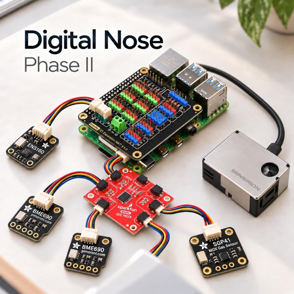
Phase I of Digital Nose was deliberately simple.
I started with one ENS160 sensor, a microcontroller and a small cloud pipeline. The idea was to find out whether a smell event that was obvious to a person could also be seen in the data.
It could.
The ENS160 reacted to changes in the air, the microcontroller collected the readings continuously, and the dashboard made it possible to compare the measurements with things such as weather, window state and manual smell reports.
That was enough to prove the basic concept, but not enough to identify a source.
A single VOC sensor can react to many things: cooking, food, cleaning products, perfume, alcohol and other compounds in the room. The response also changes with ventilation, humidity and temperature.
So Phase II had one practical objective:
Build a broader sensor array and make sure the measurements are reliable before using them for machine learning.
That sensor array is now running.
Digital Nose currently collects gas-response, particulate and environmental data from several independent sensors, stores it locally, sends it to the cloud and exposes it through the dashboard.
The ML part comes later.
For now, I want to understand the instrument.
From one sensor to several independent signals
The original Phase I ENS160 remains in place.
I did not want Phase II to replace a working acquisition path. The existing ENS160 collector, aggregator and sync services were preserved and the new sensors were added alongside them.
The array now consists of:
| Sensor | Measures | How to read it |
|---|---|---|
| ENS160 | TVOC, eCO₂ and manufacturer AQI | Processed estimates from Phase I. A TVOC peak means the chemical environment changed; it does not identify the compound. eCO₂ is an equivalent figure, not a direct CO₂ measurement. |
| BME690 #1 | Gas resistance, temperature, humidity and pressure | Gas resistance is the electrical resistance of the heated sensing layer, in ohms. Compare changes on this sensor and heater setting; neither 15 kΩ nor 30 kΩ universally means good or bad air. This unit also supplies the temperature and humidity used to compensate the SGP41. |
| BME690 #2 | Independent gas-resistance channel | The same sensor family as #1, on its own mux channel. I want to see whether the two respond similarly, or whether a stable difference is itself a useful signal. |
| SGP41 | Raw VOC and NOx | Sensirion ticks proportional to the logarithm of sensing-layer resistance. Not ppb, ppm or an air-quality index. Under manufacturer tests, ethanol lowers raw VOC ticks and NO₂ raises raw NOx ticks; mixed indoor air does not convert that cleanly. Compare against this sensor’s own baseline. |
| SPS30 | PM1, PM2.5, PM4, PM10, particle counts and typical particle size | Optical estimates of particulate mass, in µg/m³. Size fractions overlap, so they should not be added together. A short PM2.5 spike is not a WHO or UK 24-hour exposure assessment. |
The final hardware therefore measures several different properties of the same air.
That is more useful than having several sensors that all try to produce the same air-quality number.
A cooking event may create a VOC response, particulate matter, or both. Two gas sensors may react at different speeds or amplitudes. Humidity and temperature may also affect the response.
At this stage I do not know which combination will be useful for classification.
That is exactly what the next dataset is supposed to establish.
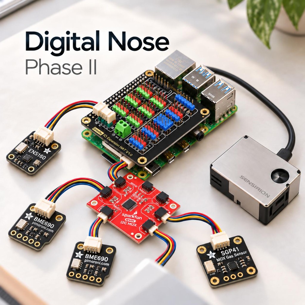
The Phase II array: ENS160 on the original I²C path, two BME690s and an SGP41 through a SparkFun multiplexer, and the SPS30 over USB.
Two BME690 sensors on one microcontroller
The first hardware problem was straightforward.
Both BME690 sensors use the same I²C address: 0x76.
They therefore cannot sit directly on the same bus and be addressed independently.
I used a TCA9548A I²C multiplexer to separate them.
The final layout is:
- BME690 #1 on MUX channel 0
- BME690 #2 on MUX channel 1
- SGP41 on MUX channel 3
- SPS30 over USB/UART
- ENS160 on the existing Phase I path
When channel 0 is selected, the microcontroller sees the first BME690 at 0x76.
When channel 1 is selected, it sees the second one at the same address.
The acquisition code also uses a shared lock around MUX access so that different sensor processes do not switch channels underneath each other.
That is the kind of issue that does not appear in a normal web application. Once several physical devices share a bus, software timing and hardware topology become part of the same problem.
The two BME690s are now producing parallel streams.
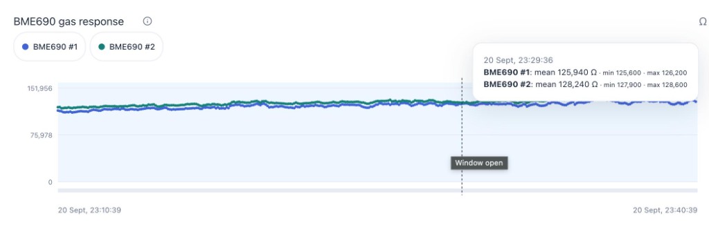
BME690 #1 and #2 over 30 minutes on 20 September, with the window open.
The two sensors follow the same shape with a small offset, around 126 kΩ and 128 kΩ. That offset may be manufacturing variation, heater state, or something useful later. I am recording it, not explaining it yet.
Connecting the SPS30
The SPS30 particulate sensor uses a different path.
I connected it through Sensirion's UART-to-USB cable and configured a stable serial-device path on the microcontroller.
I did not want the collector to depend on a temporary Linux device name such as /dev/ttyUSB0, because that name can change after a reboot or after another USB device is added.
The SPS30 adds measurements that were missing completely in Phase I.
It reports particulate mass for PM1, PM2.5, PM4 and PM10, together with particle counts and typical particle size.
For a project focused on cooking odours, this is useful because cooking does not only produce volatile gases. It can also produce particles.
Whether those particulate patterns will help distinguish one source from another is still an open question, but I can now measure them properly.
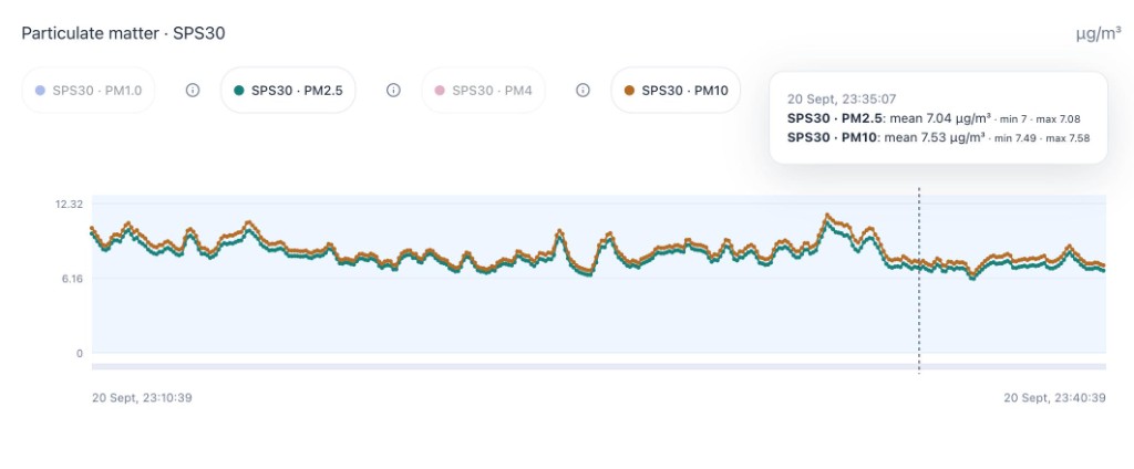
SPS30 PM2.5 and PM10 over the same half hour, both around 7 µg/m³.
They move together, which is what you would expect when the size fractions overlap. This is a live stream, not a labelled cooking event.
Using BME690 data to compensate the SGP41
BME690 #1 also provides the environmental input used by the SGP41. The SGP41's gas response depends partly on ambient temperature and humidity, so the sensor is run with compensation using the measurements from BME690 #1.
The important part here is that the SGP41 still remains its own independent gas-response channel. I am not trying to make all of the sensors produce matching numbers, just to preserve their different responses and then compare them later.
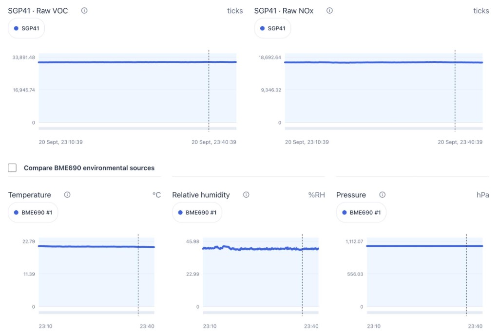
SGP41 raw VOC and NOx over the same half hour, with temperature, humidity and pressure from BME690 #1.
The gas ticks barely move, and the environmental channels are equally quiet. A flat stretch is as useful as a peak at this stage: it is a candidate baseline, not a classification.
Raw sensor values are not automatically air-quality scores
This became an important part of the dashboard work. It is easy to take every sensor value and attach a green, amber or red badge to it. In several cases that would be misleading.
The SGP41 raw VOC and NOx outputs are electrical response values. They are not direct ppm or ppb concentration measurements. The BME690 gas-resistance value is also best treated as a relative signal. There is no universal resistance threshold where one value means good air and another means unhealthy air. Particulate measurements are different because PM2.5 is a real concentration measurement, but even there the interpretation depends on the averaging period. A short PM2.5 spike should not be presented as if it were equivalent to prolonged exposure.
I changed the dashboard so that raw SGP41 and BME690 signals remain neutral.
For each displayed metric I now explain:
- what is being measured
- how the value should be interpreted
- how Digital Nose intends to use it
- what the measurement cannot establish on its own
That is useful for the dashboard, but it is also useful preparation for the ML stage. I need to know exactly what each feature represents before deciding whether it belongs in a model.
The first BME690 bug looked like a sensor problem
One of the first commissioning issues was with the two BME690 sensors. The temperature, humidity, pressure and gas readings looked reasonable, but most observations were being marked as invalid. Initially it looked as if the hardware or the driver was unstable.
The problem was in my adapter code. I was expecting the BME690 meas_index field to increment between measurements and was treating repeated values as duplicates. The driver I was actually using does not work that way in forced mode. meas_index can legitimately remain at zero.
The sensor readings were fine. My validity rule was wrong. I removed the index-based rejection and kept the checks that actually apply to the measurement: new data, heater state and gas-valid state. Both BME690 sensors then settled into stable 1 Hz streams.
This is exactly why I do not want to jump into model training yet. If I had started collecting labelled training data before finding this, part of the dataset would have contained a validity flag that described my software assumption rather than the sensor.
The SGP41 looked invisible
The SGP41 produced a different problem. It had power, but it did not appear in a generic i2cdetect scan. I tried another cable and saw the same result.
Instead of treating the scan as definitive, I initialised the sensor using its actual protocol. That worked immediately and the device returned its serial number. The sensor was healthy.
The final configuration is MUX channel 3 at address 0x59. This was a useful reminder that generic bus diagnostics are not always enough. The proper test for a device is whether it behaves correctly through the protocol it is designed to use.
SGP41 timing was more sensitive than expected
Once the SGP41 was running continuously, another issue appeared. It would produce valid readings, then occasionally throw a runtime error and return to its conditioning state. The systemd service itself had not restarted.
The issue was measurement timing. The SGP41 expects commands at approximately one-second intervals and rejects calls that arrive too close together. Because several devices share the multiplexer, one sample can sometimes be delayed slightly. The next loop iteration can then arrive too soon relative to the delayed command.
I changed the scheduler so that it controls the one-second cadence directly. If a call would happen too early, it waits. A delayed sample no longer causes the sensor to restart conditioning.
During a five-minute validation run, the SGP41 produced 336 normal readings, 10 expected startup warm-up readings and no errors after conditioning. Without that fix, a timing artefact could easily have ended up in the future dataset looking like a real environmental pattern.
Storage contention caused what looked like hardware failure
The most useful Phase II debugging session happened during reboot testing. After the microcontroller restarted, all of the sensors initially came up correctly. A short time later the SGP41 went back into warm-up and the SPS30 raised a serial exception. SQLite errors happened at roughly the same time.
My first suspicion was the hardware: USB startup behaviour, I²C instability, power, or the serial adapter. The system logs did not support that. There was no kernel USB failure, no undervoltage, no systemd restart, and the serial device remained present.
I repeated the reboot without connecting over SSH or running diagnostic commands during startup. The problem still happened.
The actual issue was the way acquisition and persistence were coupled. Sensor reads and SQLite writes shared too much of the same execution path. When SQLite stalled briefly during startup, that delay could push the sensor work beyond its deadline. The runtime would then react as if the hardware itself had failed. That meant a temporary database problem could close and reopen a perfectly healthy sensor.
I changed the lifecycle around this. Persistence now happens outside the sensor deadline. If SQLite is temporarily unavailable, the current observation is held in memory and retried using bounded backoff. A new reading does not silently overwrite the pending one. The sensor remains open unless there is an actual sensor or communication failure. Storage recovery and hardware recovery are now separate paths.
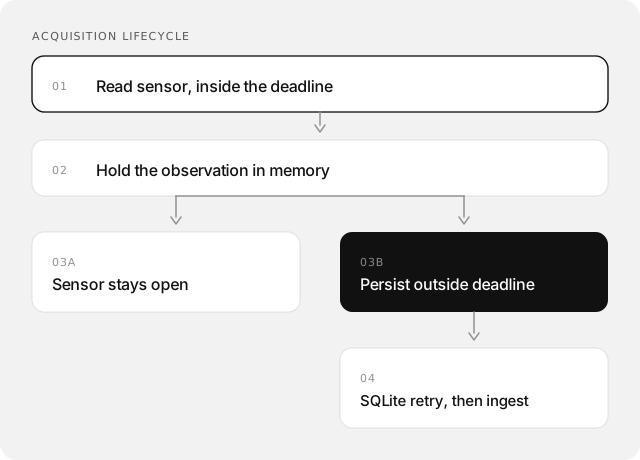
If SQLite stalls, the current observation is retried. A new reading does not silently overwrite the pending one. The sensor is closed only for an actual sensor or communication failure. Storage recovery and hardware recovery are now separate paths.
I then repeated the reboot test. There was still a short 6–7 second period of SQLite contention early in startup, but this time it stayed a storage problem. The SGP41 did not recondition. The SPS30 did not throw another serial exception. No sensor service restarted. The observations remained ordered and contiguous.
That was a much more useful acceptance test than simply reading one value from each sensor manually.
A reserved SPS30 status bit
The SPS30 produced one more interesting commissioning issue. Some observations contained a device status value of 1048576. At first glance it looked like a hardware fault. It was actually bit 20, which is reserved.
The documented SPS30 public fault bits are for speed, laser and fan errors. I now store the raw status exactly as returned, but the validity logic only reacts to documented fault bits. Again, the raw data stays intact while the interpretation is handled separately.
Independent acquisition and durable local queues
Phase II also changed the way observations move through the system. Each new sensor has its own acquisition process and its own SQLite outbox. Observations are recorded independently, with their own timestamps and sequence numbers.
They are then published to:
POST /api/ingest/sensors
The cloud side separates:
- sensor registrations
- raw observations
- derived values
I prefer this to constructing one large "sensor array row" on the microcontroller. The sensors do not all sample at exactly the same instant. They have different warm-up behaviour and different failure modes. Keeping the original observations independent means I can decide later how to align them into time windows without losing what was actually recorded.
The SPS30 production path was also tested with a controlled observation before the queue was allowed to drain normally.
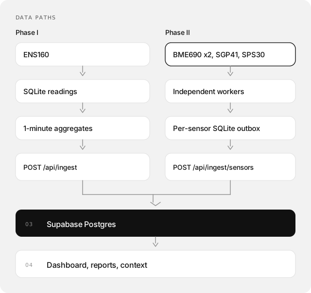
Observations stay independent: their own timestamps, sequence numbers and failure modes. Alignment into time windows can happen later, without losing what was actually recorded.
This is the same edge-first idea as Phase I. If Wi-Fi disappears, sensing should continue. If the API fails, sensing should continue. The new sensors get the same treatment, just without being forced into one shared row.
The dashboard now reflects the full array
The Phase I dashboard was mainly designed around ENS160 data. Phase II adds charts for particulate matter, gas response and environmental measurements. PM2.5 is now part of the main summary. Pressure is displayed in hPa rather than Pa, while the stored measurement remains unchanged.
Metric labels, units, explanations and limitations are handled centrally so that the same measurement is described consistently throughout the interface. I also changed timeframe navigation to refresh charts in the background instead of reloading the whole view. The UI changes are relatively small compared with the hardware work, but they make it much easier to inspect several sensors at once and compare events across the same time period.
The original ENS160 view is still the place where a smell report, occupancy, window state and wind sit on the same timeline.
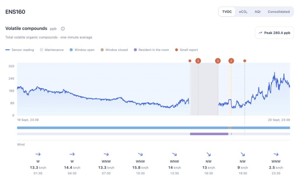
24-hour ENS160 TVOC from 19–20 September. Peak 280.4 ppb, with smell reports, occupancy, maintenance and wind.
I have not yet lined this window up against the new BME690, SGP41 and SPS30 channels. That alignment is the gathering work, not a result.
What I want to collect now
Phase II gives me the platform needed to start building a calibration dataset.
The traces above are the start of that dataset. They are what the instrument produced while I was still commissioning it. I have not yet run controlled sources against them, and I am not treating a quiet half hour or a single TVOC peak as a conclusion.
The useful information will probably come from combinations of measurements rather than any single sensor value.
For each event I can now look at:
- ENS160 TVOC
- ENS160 eCO₂
- ENS160 AQI
- BME690 #1 gas resistance
- BME690 #2 gas resistance
- SGP41 raw VOC
- SGP41 raw NOx
- PM1
- PM2.5
- PM4
- PM10
- particle counts
- typical particle size
- temperature
- humidity
- pressure
- rate of change
- response delay between sensors
- recovery time
- window state
- manual smell reports
- wind direction
- wind speed
- rainfall and other weather context
I am particularly interested in the shape of an event. A useful signature may turn out to be something like:
- VOC rises first
- PM2.5 follows 30 seconds later
- BME690 #1 changes more strongly than #2
- humidity remains flat
- the signal decays over 20 minutes
Another source may create a completely different sequence. I do not know yet which of those relationships are repeatable. The next stage is to find out.
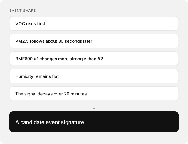
This is a hypothesis, not a result. Another source may create a completely different sequence. The next dataset is supposed to show which relationships repeat.
Why I am not training a model yet
It would be easy to start now. I already have several sensors, cloud storage, a dashboard and manual smell reports. I could label a few periods as restaurant, label some others as normal, train a classifier and display a confidence score.
The problem is that Phase II has already shown several ways in which that dataset could have been wrong. The BME690 validity flag was initially wrong because of my adapter logic. The SGP41 could re-enter conditioning because of scheduler timing. Storage contention could previously trigger what looked like a sensor failure. The SPS30 exposed a reserved status bit that could easily have been classified incorrectly.
Those are software and commissioning artefacts. I do not want the model learning them.
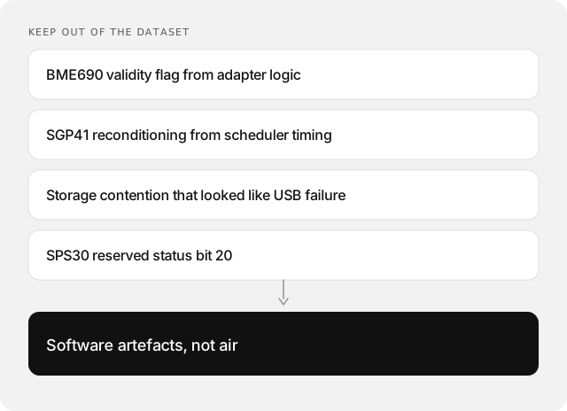
These would have been easy to treat as environmental patterns. They described my code, not the room. A classifier cannot tell the difference. The dataset has to, before training starts.
Before training anything, I want answers to a few basic questions.
Baseline stability
How stable is each sensor when nothing interesting is happening? Does the baseline move during the day? Does it drift over several days?
Repeatability
If I introduce the same controlled source several times, do I see a similar response? If not, what changed?
Environmental effects
How much of the gas response can be explained by temperature or humidity? How much does ventilation affect the shape and duration of an event?
Cross-sensor behaviour
Do the two BME690s respond similarly? If they differ, is that difference stable and useful, or simply manufacturing variation?
Particulate response
Do cooking events repeatedly produce a PM pattern? Do non-cooking VOC sources produce the same one?
Sensor artefacts
Can warm-up, temporary storage stalls or communication recovery be identified reliably and excluded from training?
Until I know those things, a model accuracy number would not tell me much.
Avoiding shortcuts in the ML stage
There is another problem I want to avoid. A classifier does not know what I intend it to learn.
If restaurant events mostly happen in the evening, a model may learn the time of day. If they happen only when the wind comes from one direction, it may rely too heavily on weather. If the strongest manually labelled events also have the largest VOC peaks, it may just learn signal magnitude.
Any of those could produce a good-looking validation result without solving the actual problem. The commissioning work already gave me concrete examples of why the dataset needs to be inspected carefully before training. The next phase therefore starts with calibration and experiment design rather than a model. This is the same progression I described in Phase I: instrument, observe, understand failure modes, improve sensing, then model. Not sensor, then AI.
Phase III: SSM
Phase III will introduce SSM — Smell Sensing Model. The first experiments will be fairly narrow.
I want to test whether:
- unusual events can be separated from the normal baseline;
- similar events naturally form recurring clusters;
- known restaurant or cooking events can eventually be distinguished from other indoor or outdoor sources.
From there, the system can grow into:
- anomaly detection
- event start/end detection
- recurring signature clustering
- source classification
- intensity estimation
- unknown-event rejection
Unknown events are important. I do not want every new smell to be forced into the closest known category. If the measurements do not resemble anything in the training set closely enough, the correct result may simply be unknown.
Inference can eventually run on the microcontroller, but there is no reason to optimise that yet. At the moment, collecting clean data is more valuable.
Where Phase II leaves the project
Phase II has taken Digital Nose from one general-purpose gas sensor to a heterogeneous sensing platform.
The microcontroller now runs the original ENS160 pipeline alongside:
- two BME690 gas-response channels
- SGP41 VOC/NOx sensing
- SPS30 particulate sensing
- temperature, humidity and pressure measurements
- independent acquisition services
- durable local queues
- production cloud ingestion
- automatic recovery after reboot
The production topology and the microcontroller configuration are now aligned, and the complete array is streaming valid observations alongside the existing Phase I data. The commissioning work was at least as useful as adding the sensors themselves. It exposed problems in validity logic, timing, storage coupling and status interpretation before those problems could become part of the ML dataset.
For now, I am going to leave the array running and collect calibration data. I want to establish normal behaviour, compare controlled events with real nuisance events, measure drift, and see which responses repeat across different environmental conditions. Once I know which parts of the signal are stable and which are caused by the sensors, software or environment, Phase III can start testing whether the recurring patterns are actually separable.
Until then, training a classifier would be mostly guessing with more mathematics.
Leaving the array running exposed a different problem first. The raw stream was growing faster than an operational database should, which is what Digital Nose - Phase III: Building the Dataset Before the Model had to fix.
Digital Nose is a Physical AI project: sense the real world first, then decide whether a model belongs in the loop. More on my profile.