Digital Nose - Phase I: From Hardware to Real-World Data

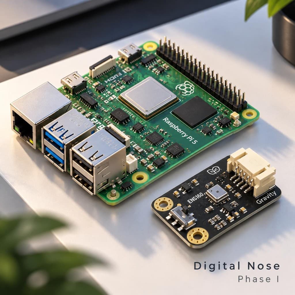
I really enjoy tackling complex problems that let me use all my engineering skills, from hardware and electronics to embedded software, software engineering, and AI. This weekend's project is a perfect example. It requires me to work across all these areas as I move from Phase I to Phase III.

I love rapid prototyping and creating an MVP with minimal effort, so I’m excited to share how this project turned out!

Digital Nose started with a simple real-world problem. Cooking smells from a nearby restaurant occasionally drift towards my building and into the room where I work. Smell is obvious to a human when it happens, but surprisingly difficult to record objectively afterwards. The useful question was therefore whether I could build a system that records enough physical and contextual information to understand what actually happened around an odour event, how the environment changed, and whether similar events could eventually be recognised again.

So Phase I had one purpose: build the instrumentation first. Not machine learning. Not smell classification. Not an elaborate electronic nose. I wanted a reliable system capable of collecting a continuous physical signal and putting it next to enough contextual information to make that signal useful.

This is also very close to the principle I wrote about in Start small: the first version should reduce uncertainty, not try to become the final product immediately. That system is now running.

Phase I: the system

The initial architecture is deliberately simple. At the physical layer I am using an ENS160 gas sensor connected through I²C to an edge computer. The sensor provides processed measurements including TVOC, equivalent CO₂ and an air-quality index.

The important limitation is that this is not a chemical identification system. A TVOC value does not tell me this is restaurant smell, and it cannot prove the source of an event. For Phase I, the sensor only needs to tell me that the chemical environment around it changed in a measurable way.

The first hardware path looked like this:

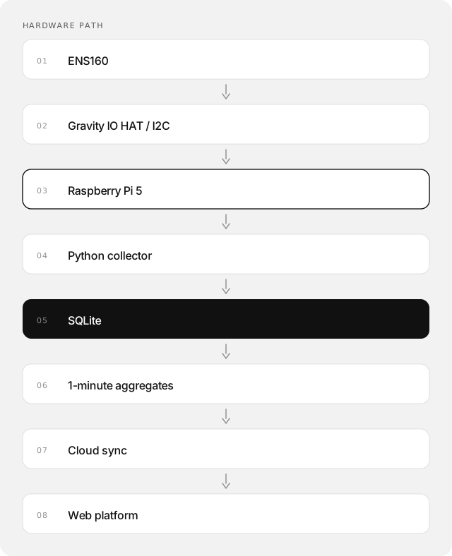
The original setup deliberately treated the Pi as an independent edge appliance. It reads the sensor every five seconds, stores the raw measurements locally, produces a derived one-minute dataset and keeps running regardless of whether the cloud application is available. That separation became one of the most important Phase I architecture decisions.

Start with the edge, not the dashboard

It would have been very easy to start with the web application. I deliberately did not. If Wi-Fi disappears, sensing should continue. If the API fails, sensing should continue. If the frontend is redeployed, sensing should continue. The physical system should not care.

Every five seconds, the collector writes a raw measurement into SQLite. A second process derives one-minute aggregates for the dashboard and cloud layer. The raw data is retained separately rather than being replaced by the aggregated dataset.

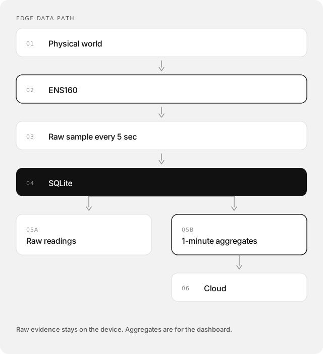
The one-minute dataset exists for efficiency and visualisation. It does not improve sensor accuracy, and it does not replace the raw evidence. The complete five-second dataset remains on the device for later analysis, because UI decisions should never destroy experimental data.

Proving the hardware path first

Before writing the collector, I verified the hardware independently. The I²C bus exposed:

• 0x10 → Gravity IO HAT
• 0x53 → ENS160

I then ran the vendor example directly before writing any of my own application logic. That follows a simple debugging rule I like: prove each layer independently before combining them. Once the vendor example was returning sensible values, I knew that the physical connection, I²C bus, sensor address and basic library integration were all working.

The sensor also exposed another important aspect of physical computing: warm-up state. The ENS160 initially reported startup status and later transitioned into normal operation once it had warmed up. Software may start instantly. Sensors do not always behave that way.

The Python collection layer

Once the hardware path was stable, I wrapped the vendor library behind a very small interface. The sensing code is intentionally boring:

class ENS160Sensor:
    def __init__(self):
        self.sensor = DFRobot_ENS160_I2C(
            i2c_addr=0x53,
            bus=1
        )
 
    def initialise(self):
        while not self.sensor.begin():
            time.sleep(3)
 
    def read(self):
        return {
            "sensor_status": self.sensor.get_ENS160_status(),
            "aqi": self.sensor.get_AQI,
            "tvoc_ppb": self.sensor.get_TVOC_ppb,
            "eco2_ppm": self.sensor.get_ECO2_ppm,
        }

The implementation separates sensor access, persistence, collection and aggregation into separate Python modules rather than placing the whole device into one script. The collector itself simply reads the sensor, timestamps the result in UTC, writes the values to SQLite and sleeps until the next sample.

while True:
    reading = sensor.read()
    timestamp = utc_now()
 
    insert_reading(
        recorded_at_utc=timestamp,
        tvoc_ppb=reading["tvoc_ppb"],
        eco2_ppm=reading["eco2_ppm"],
        aqi=reading["aqi"],
        sensor_status=reading["sensor_status"],
    )
 
    time.sleep(5)

The production implementation also catches individual read failures so a single bad sample does not stop the acquisition process. A sensor collector should not be clever. It should collect.

Raw evidence first

The local database has two main datasets. The first stores every raw sample:

CREATE TABLE sensor_readings (
    id INTEGER PRIMARY KEY AUTOINCREMENT,
    recorded_at_utc TEXT NOT NULL,
    tvoc_ppb INTEGER NOT NULL,
    eco2_ppm INTEGER NOT NULL,
    aqi INTEGER NOT NULL,
    sensor_status INTEGER NOT NULL,
    synced_at_utc TEXT
);

The second stores one-minute aggregates:

CREATE TABLE minute_aggregates (
    minute_start_utc TEXT PRIMARY KEY,
    tvoc_mean REAL NOT NULL,
    tvoc_min INTEGER NOT NULL,
    tvoc_max INTEGER NOT NULL,
    eco2_mean REAL NOT NULL,
    eco2_min INTEGER NOT NULL,
    eco2_max INTEGER NOT NULL,
    aqi_max INTEGER NOT NULL,
    sample_count INTEGER NOT NULL
);

For each minute I retain mean, minimum and maximum values rather than only an average. That matters because a short, sharp event could disappear inside a mean value while still being visible in the spread. The database therefore preserves both the compact dataset needed by the web application and the raw data needed later for proper analysis.

Making the device behave like an appliance

The next requirement was that the system should work without an SSH session or a manual command. Both Python processes therefore run under systemd. The collector is configured to start automatically and restart after a failure:

[Service]
Type=simple
User=diginose
WorkingDirectory=/home/diginose/digital-nose
ExecStart=/usr/bin/python3 -u /home/diginose/digital-nose/collector.py
Restart=always
RestartSec=5

The aggregator runs as a separate service, which means the device can reboot and resume acquisition without intervention. For me, that is the difference between successfully reading a sensor and actually building an instrument.

Building the web layer around the experiment

Once the acquisition layer was stable, I moved outward. The original edge guide ends at the point where the architecture becomes:

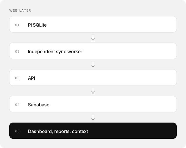
The design deliberately separates device telemetry from manual observations. Human reports are context or labels, not sensor truth, and should never overwrite the physical data. That architecture is now reflected in the web platform.

The dashboard places the sensor signal on the same timeline as window state, room occupancy, smell reports, wind speed and direction, humidity, temperature, rainfall and pressure. That is where the raw sensor value becomes useful. A number by itself is not particularly interesting. An event with context is.

This is also where Digital Nose connects directly with the MVP approach I described in Your first MVP. The point of a first version is to test one central idea and make it cheap to change if the original assumption proves wrong. That is exactly what happened here.

What the first real data is showing

Once the system had been running in the actual environment, the interesting part started. These are still early observations and working hypotheses, not controlled scientific conclusions, but they have already changed how I think Phase II needs to work.

Observation 1: the room appears to exchange air effectively

The first thing visible in the data is how quickly larger TVOC excursions can move back towards the previous baseline.

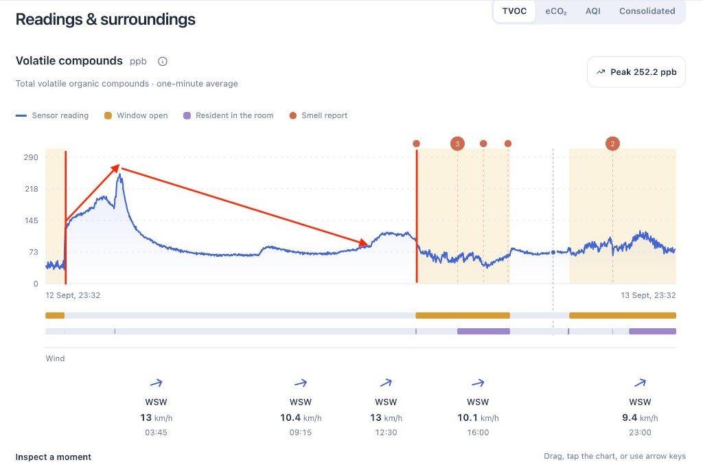
A 24-hour TVOC trace. After the plume arrives, the concentration falls back towards the previous baseline rather than remaining elevated.

I would not claim from one VOC sensor that I have formally measured the building's ventilation performance, but the observed behaviour is consistent with a room that is continuously exchanging air rather than trapping volatile compounds indefinitely. That was useful immediately: the system was already telling me something about the environment that was difficult to judge from smell alone.

Observation 2: the open window makes measurement harder

The sensor is positioned close to the window because that is where the external smell enters. That sounds like the obvious location, but it also creates a measurement problem.

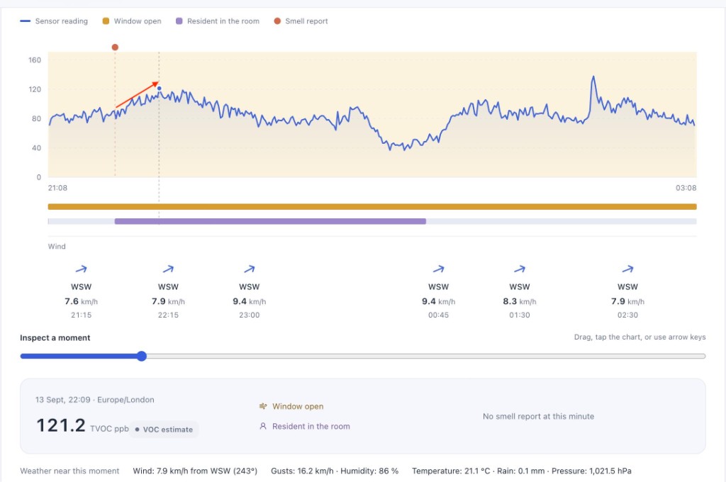
Window open at 22:09. A noticeable plume, but TVOC only 121.2 ppb.

I walked into the room to a strong plume. The window was open, the smell was obvious, and the sensor only reached 121.2 ppb — a peak, but not a strong one.

With the window open, outside air is continuously moving across the sensor. When the cooking smell arrives, small TVOC peaks are visible, but the sample around the sensor is simultaneously being refreshed. The plume arrives, the sensor responds, and the surrounding concentration changes again as new air passes through.

This means the airflow that is good for the room can simultaneously make the event harder to isolate. One of the most useful Phase I lessons is therefore that sensor placement and airflow are part of the measurement system.

Observation 3: closing the window can make an event much clearer

The opposite behaviour is even more interesting. When a strong gust brings the cooking smell into the room and the window is then closed, the local air is no longer being refreshed as quickly, and the event can become much more visible in the sensor data. In that same 24-hour window the dashboard records a peak of 252.2 ppb TVOC. At the selected moment the window is closed, while the contextual data shows wind from WSW at approximately 14 km/h, gusts of 28.8 km/h, together with humidity, temperature, rainfall and atmospheric pressure. This is exactly why I built the contextual layer. 252.2 ppb by itself is just a number. The surrounding sequence is much more interesting: a plume arrives, the environment changes, the window state changes, the local concentration rises and the signal then evolves over time.

That still does not prove that the restaurant caused that specific peak. Correlation is not source attribution. But it turns a subjective smell event into recorded physical evidence that can actually be investigated.

The airflow problem changes the future ML problem

The early data already shows why a naive classifier would fail. A clearly noticeable odour at an open window may produce only a modest TVOC change because the sensor is continuously exposed to moving air. The same incoming air, once partially contained by closing the window, can produce a much larger response. So signal magnitude alone cannot become the classifier.

A useful future model will need to consider the shape and context of the event: sensor response, rate of change, airflow, window state, weather, other sensor modalities and time history. This is one of the main reasons I wanted real measurements before touching machine learning. The environment is already showing me which assumptions would have been wrong.

Observation 4: one sensor is not enough

This is the most important Phase I conclusion. The ENS160 works: it responds to changes in the surrounding air and provides useful time-series data. But a general TVOC response is not sufficiently specific to identify the source of an event. A peak can tell me something changed. It cannot reliably tell me what changed.

That means Phase II should not simply be a better dashboard or a smarter algorithm over the same signal. It needs more independent physical information.

What Phase I actually accomplished

The purpose of this phase was not to prove that my original idea was correct. It was to reduce uncertainty. So far, Phase I has established that:

• the edge acquisition pipeline can run continuously
• the sensor responds to real environmental changes
• those changes can be aligned with window state and weather
• airflow materially affects the shape and magnitude of the signal
• one general TVOC measurement is not specific enough for source classification

That is a useful result. The first version has already changed what I think the second version should be. That is the same basic principle behind Start small and Your first MVP: the first version is there to produce evidence and expose wrong assumptions cheaply, not to demonstrate that the founder was right all along.

What Phase II needs

The next improvement is not more software. It is more sensing. The direction is a heterogeneous sensor array combining several independent signals rather than relying on one TVOC value.

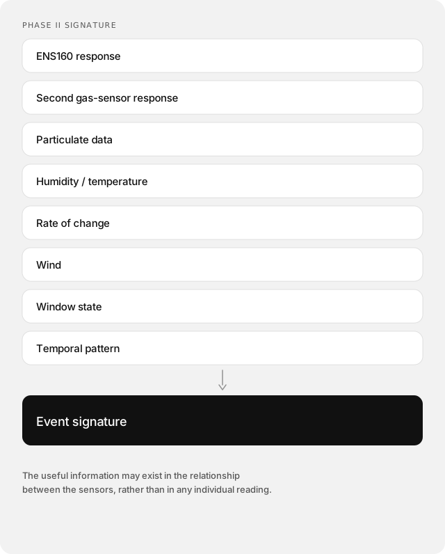
The useful information may exist in the relationship between the sensors, rather than in any individual reading. A cooking plume may produce a combination of gas response, particulates, environmental conditions and temporal behaviour that becomes significantly more characteristic than TVOC alone. That is the experiment for Phase II.

Why ML comes later

It would be easy to build a classifier now. I could take several peaks, label some as restaurant-related, label other periods as normal and train something that produces a confidence score. That would look impressive. It would probably also be wrong. The current dataset is telling me that the measurement layer still needs more information.

So the progression remains:

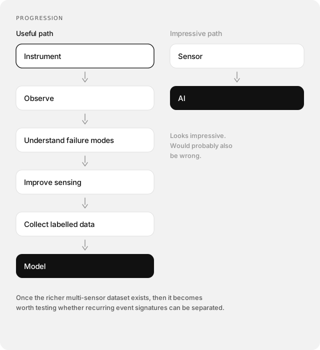
Once the richer multi-sensor dataset exists, then it becomes worth testing whether recurring event signatures can be separated reliably.

Phase I conclusions

The current conclusions are straightforward. The air exchange in the room appears to be working: larger changes tend to reduce again rather than remain permanently elevated, although I am not treating a VOC sensor as a formal ventilation measurement. An open window makes the incoming smell harder to measure than I initially expected, because the sensor is continuously exposed to moving air and its local sample is constantly being refreshed. A strong plume followed by closing the window can produce a much larger and clearer response. That gives me a useful clue about concentration, airflow and sensor positioning, although it still does not establish source attribution.

One TVOC sensor is not enough. It is useful for detecting that something changed, but it is not sufficiently specific for determining what caused the change. Phase II therefore needs a proper sensor array before Phase III ML becomes worthwhile.

That is exactly what an MVP should do. It should not prove that the original idea was right. It should tell you what to build next. Digital Nose Phase I has done that.

Digital Nose · Open-source repository